Iris Dataset#
準備#
必要なパッケージを読み込む.
using Flux, DataFrames, Random, RDatasets
using Flux: params, Data.DataLoader
using MLDataUtils: shuffleobs
Iris データの読み込み#
iris = dataset("datasets", "iris")
まずは, Iris データの構造を見てみる.
julia> describe(iris, :all)
5×16 DataFrame
 Row │ variable     mean     std       min     q25     median  q75     max        sum     nunique  nuniqueall  nmissing  nnonmissin ⋯
     │ Symbol       Union…   Union…    Any     Union…  Union…  Union…  Any        Union…  Union…   Int64       Int64     Int64      ⋯
─────┼───────────────────────────────────────────────────────────────────────────────────────────────────────────────────────────────
   1 │ SepalLength  5.84333  0.828066  4.3     5.1     5.8     6.4     7.9        876.5                    35         0          15 ⋯
   2 │ SepalWidth   3.05733  0.435866  2.0     2.8     3.0     3.3     4.4        458.6                    23         0          15
   3 │ PetalLength  3.758    1.7653    1.0     1.6     4.35    5.1     6.9        563.7                    43         0          15
   4 │ PetalWidth   1.19933  0.762238  0.1     0.3     1.3     1.8     2.5        179.9                    22         0          15
   5 │ Species                         setosa                          virginica          3                 3         0          15 ⋯
これでは全て表示されないので外部ファイルにリダイレクトする.
description = describe(iris, :all)
open("describe_iris.txt", "w") do file
    write(file, string(description))
end
describe_iris.txt は以下の通り.
5×16 DataFrame
 Row │ variable     mean     std       min     q25     median  q75     max        sum     nunique  nuniqueall  nmissing  nnonmissing  first   last       eltype
     │ Symbol       Union…   Union…    Any     Union…  Union…  Union…  Any        Union…  Union…   Int64       Int64     Int64        Any     Any        DataType
─────┼───────────────────────────────────────────────────────────────────────────────────────────────────────────────────────────────────────────────────────────────────────────────────
   1 │ SepalLength  5.84333  0.828066  4.3     5.1     5.8     6.4     7.9        876.5                    35         0          150  5.1     5.9        Float64
   2 │ SepalWidth   3.05733  0.435866  2.0     2.8     3.0     3.3     4.4        458.6                    23         0          150  3.5     3.0        Float64
   3 │ PetalLength  3.758    1.7653    1.0     1.6     4.35    5.1     6.9        563.7                    43         0          150  1.4     5.1        Float64
   4 │ PetalWidth   1.19933  0.762238  0.1     0.3     1.3     1.8     2.5        179.9                    22         0          150  0.2     1.8        Float64
   5 │ Species                         setosa                          virginica          3                 3         0          150  setosa  virginica  CategoricalValue{String, UInt8}
ちなみに, これではアヤメの品種がすべて表示されていいないため, 以下のようにする.
julia> unique(iris.Species)
3-element Vector{String}:
 "setosa"
 "versicolor"
 "virginica"
これにより, アヤメの品種として setosa , versicolor , virginica が含まれることが確認できた.
アヤメの品種 (setosa , versicolor , virginica) を特定するためのデータとして SpealLength , SpealWodth , PetalLength , PetalWidth が存在している.
目的変数と説明変数の定義#
目的変数として SpealLength , SpealWidth , PetalLength , PetalWwidth , 説明変数として Species を選択する.
X = select(iris, Not(:Species)) |> Matrix
y = iris[:, :Species]
なお, X は DataFrame であるが, 今後の処理のため, Matrix に変換している.
訓練データとテストデータに分離#
訓練データとテストデータに分割する. ここでは, 「訓練データ:テストデータ = 7:1」で分割する.
function partition(data, labels, at = 0.7)
    n = size(data, 1)
    idx = shuffle(1:n)
    train_idx = view(idx, 1:floor(Int, at*n))
    test_idx = view(idx, (floor(Int, at*n)+1):n)
    return data[train_idx, :], labels[train_idx], data[test_idx, :], labels[test_idx]
end

x_train, y_train, x_test, y_test = partition(X, y, 0.7)
One-Hot エンコーディング#
目的変数を数値化するために, One-Hot エンコーディングを行う.
y_train = Flux.onehotbatch(y_train, unique(iris.Species))
y_test = Flux.onehotbatch(y_test, unique(iris.Species))
データローダ作成#
batch_size = 16
train_dl = DataLoader((x_train', y_train), batchsize=batch_size, shuffle=true)
test_dl = DataLoader((x_test', y_test), batchsize=batch_size)
モデル定義#
以下のようなモデルを定義する.
入力層:
入力:\(x\in\mathbb{R}^{4}\)
出力:\(h^{(1)}=\mathrm{ReLU}(\mathbf{W}^{(1)}+b^{(1)}), \quad \mathbf{W}^{(1)},\, b^{(1)}\in\mathbb{R}^{32}\)
活性化関数:\(\mathrm{ReLU}(z)=\max(0,z)\)
中間層:
入力:\(h^{(1)}\in\mathbb{R}^{32}\)
出力:\(h^{(2)}=\mathbf{W}^{(2)}h^{(1)}+b^{(2)}, \quad \mathbf{W}^{(2)}\in\mathbb{R}^{3\times32},\, b^{(2)}\in\mathbb{R}^{3}\)
活性化関数:なし
出力層:
入力:\(h^{(2)}\in\mathbb{R}^{3}\)
出力:\(\hat{y}=\mathrm{softmax}(h^{(2)})\)
model = Chain(
    Dense(4, 32, relu),
    Dense(32, 3),
    softmax
)
損失関数#
損失関数にはクロスエントロピーを利用する.
クロスエントロピー:
loss(x, y) = Flux.crossentropy(model(x), y)

train_losses = []
test_losses = []
train_acces = []
test_acces = []
最適化手法#
ここでは, 最適化手法として ADAM を選択する.
ADAM:
lr = 0.001
opt = ADAM(lr, (0.9, 0.999))
Callbacks#
train!() 内で呼び出す callbacks を作成する.
function loss_all(data_loader)
    return sum([loss(x, y) for (x, y) in data_loader]) / length(data_loader)
end

function acc(data_loader)
    f(x) = Flux.onecold(cpu(x))
    acces = [sum(f(model(x)) .== f(y)) / size(x, 2) for (x, y) in data_loader]
    return sum(acces) / length(data_loader)
end

callbacks = [
    () -> push!(train_losses, loss_all(train_dl)),
    () -> push!(test_losses, loss_all(test_dl)),
    () -> push!(train_acces, acc(train_dl)),
    () -> push!(test_acces, acc(test_dl)),
]
loss_all() は損失の和を返し, acc() は正答率を返す.
訓練#
モデルの特訓を行う. なお, 特訓に関して, 全データでの特訓を epochs 回行う.
ps = Flux.params(model)

epochs = 100
for epoch in 1:epochs
    Flux.train!(loss, ps, train_dl, opt, cb = callbacks)
end
結果の表示#
println("Train Error: $(loss_all(train_dl))")
println("Test Error: $(loss_all(test_dl))")
println("Train Accuracy: $(acc(train_dl))")
println("Test Accuracy: $(acc(test_dl))")
例として, 周回数を \(100\) としたときの結果を以下に示す.
Train Error: 0.24635728

Test Error: 0.2152909

Train Accuracy: 0.9732142857142857

Test Accuracy: 0.9583333333333334
予測の例#
予測の一例を以下に示す.
pred = []
truth = []
for i in 1:length(x_test[:, 1])
    push!(pred, f(model(x_test[i, :])))
    push!(truth, f(y_test[:, i]))
end
julia> pred'
1×45 adjoint(::Vector{Any}) with eltype Any:
 3  2  2  3  2  3  3  3  3  3  1  3  3  1  2  2  3  2  2  2  2  1  1  1  2  2  1  1  1  1  2  3  2  1  1  3  3  3  2  3  3  3  1  2  1

julia> truth'
1×45 adjoint(::Vector{Any}) with eltype Any:
 3  2  2  3  2  3  2  3  3  3  1  3  3  1  2  2  3  2  2  2  2  1  1  1  2  2  1  1  1  1  2  3  2  1  1  3  3  3  2  3  3  3  1  2  1
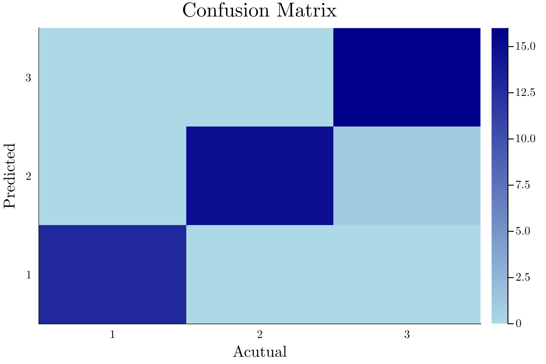
上記では, 結果を見やすくするためにあえて転置している. 上記の結果を混同行列の表にしたものを以下に示す.
julia> ConfusionMatrices.confmat(truth, pred)
          ┌──────────────┐
          │ Ground Truth │
┌─────────┼────┬────┬────┤
│Predicted│ 1  │ 2  │ 3  │
├─────────┼────┼────┼────┤
│    1    │ 13 │ 0  │ 0  │
├─────────┼────┼────┼────┤
│    2    │ 0  │ 15 │ 1  │
├─────────┼────┼────┼────┤
│    3    │ 0  │ 0  │ 16 │
└─────────┴────┴────┴────┘
また, heatmap にしたものを以下に示す.
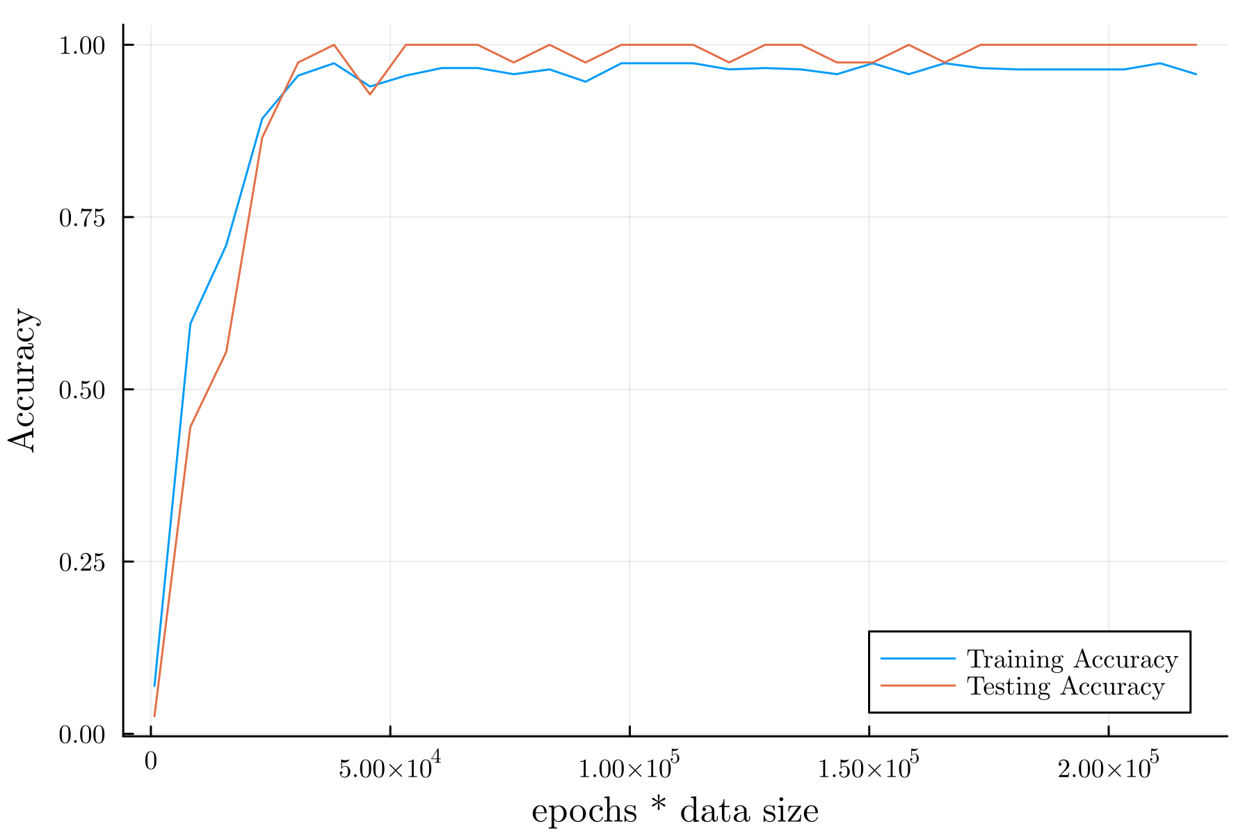
最終的な結果#
Loss:
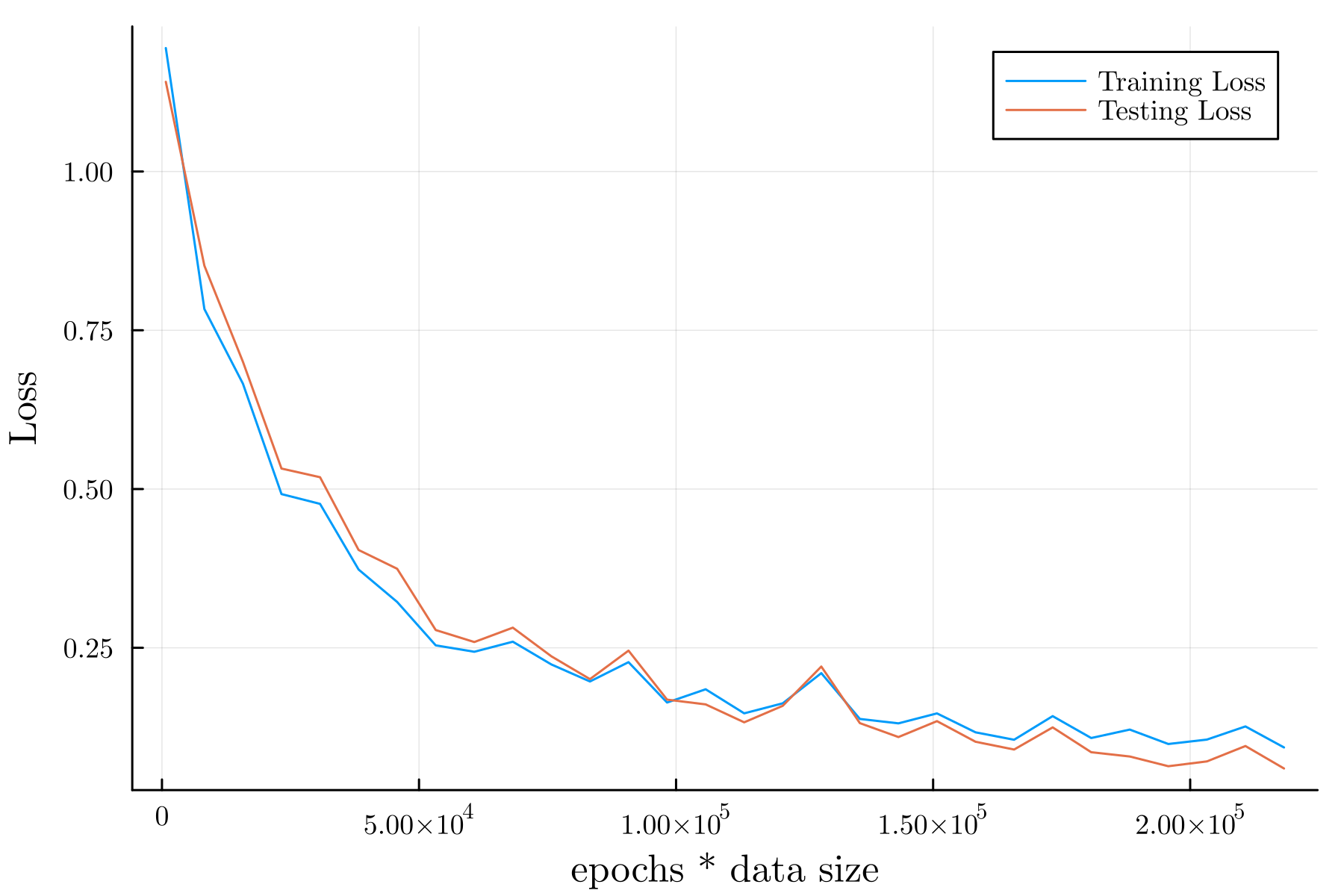
Accuracy:
参考文献#
Luke Floden, "Deep learning on "the iris data-set" in Julia", DEV, 2020-11-10, https://dev.to/bionboy/deep-learning-on-the-iris-data-set-in-julia-3pbe, (2024-06-17 参照).